Agentic AI Marketing Risk: An OpenClaw Study

Can We Trust Agentic AI to Run Marketing Campaigns Without Oversight?

A 60-day OpenClaw study finds higher detector-defined manipulation-risk signals under moderate and high optimization pressure in a multi-agent marketing workflow.

Artificial intelligence can now do more than produce a single advertisement on demand. In an agentic marketing workflow, one AI agent can draft campaign copy, another can adjust campaign objectives, and another can evaluate what the system produces. That division of labor can make marketing automation more capable—but it also creates a governance problem.

What happens when humans, business objectives, or other AI agents push the system harder to convert?

Our new open-access paper examines that question using OpenClaw, a role-based agent environment in which a Content Creator, Campaign Optimizer, and Analytics Reporter worked together across three optimization-pressure regimes.

Read the open-access paper

At a glance

Platform: OpenClaw
Study period: 60 simulated days
Scale: 1,620 experimental trials
Agent roles: Content Creator, Campaign Optimizer, and Analytics Reporter
Pressure regimes: baseline, moderate pressure, and high pressure
Measured signals: urgency exploitation, authority manipulation, and emotional coercion
Main result: moderate and high pressure exceeded baseline; moderate pressure had the highest observed mean, but moderate and high were not statistically distinguishable

Overview of the OpenClaw study. Both moderate- and high-pressure regimes produced higher detector-defined manipulation-risk signals than baseline. Moderate pressure produced the highest observed mean, but it was not statistically distinguishable from high pressure.

Why optimization pressure matters

Marketing systems are usually evaluated against commercial objectives: engagement, conversion, campaign performance, and brand consistency. In a conventional workflow, people decide how aggressively to pursue those objectives and review the resulting messages before publication.

Agentic systems can distribute those decisions across multiple AI roles. A campaign-optimization agent may prioritize conversion. A content-generation agent may translate that objective into persuasive language. An analytics agent may then evaluate the output and provide feedback. The final message is therefore shaped not only by the language model, but also by the pressure encoded in the workflow.

We use the term ethical compliance drift for movement away from acceptable persuasion and toward detector-defined manipulation-risk signals as operating pressure changes. The question is not whether every persuasive message is unethical. The question is whether stronger optimization pressure changes the kinds of persuasive tactics that appear in generated content.

What we tested in OpenClaw

The study modeled a three-agent AI marketing team:

Content Creator — generated marketing copy from a fixed pool of prompt contexts.
Campaign Optimizer — applied the pressure regime and objective configuration.
Analytics Reporter — evaluated outputs, recorded monitoring signals, and supplied feedback through the shared workflow.

The same model backend, agent roles, prompt pool, and monitoring process were held constant. What changed was the optimization-pressure regime:

Baseline: engagement, quality, and brand objectives without conversion pressure.
Moderate pressure: conversion pressure was introduced while quality and brand objectives remained active.
High pressure: conversion received the largest weight and was combined with an aggressive-adaptation term.

This distinction matters because the study compares predefined operating regimes. The high-pressure setting was a bundled configuration, not a pure one-variable increase from the moderate setting.

How we measured manipulation-risk signals

The generated messages were evaluated with a transparent rule-based detector. It recorded three categories of persuasive pressure:

Urgency Exploitation Score (UES)

UES captures language associated with artificial scarcity, countdown pressure, limited-time framing, and fear of missing out.

Authority Manipulation Index (AMI)

AMI captures unsupported expertise, inflated credibility, pseudoscientific framing, exaggerated endorsements, and similar authority cues.

Emotional Coercion Score (ECS)

ECS captures fear, guilt, regret framing, identity pressure, and social-conformity pressure.

The three components were combined into a bounded composite manipulation-risk score. These scores are detector-defined indicators. They are not direct measurements of consumer harm, deception, legal violations, or actual changes in consumer behavior.

The main result: pressure mattered, but the pattern was not linear

Optimization pressure produced a statistically reliable but small overall effect on manipulation-risk scores.

The observed condition means were:

Baseline: 0.305
Moderate pressure: 0.367
High pressure: 0.351

Both pressure conditions exceeded baseline. Moderate pressure produced the highest observed mean, but the moderate- and high-pressure conditions were not statistically distinguishable in the pairwise comparison.

That qualification is essential. The paper does not establish that moderate pressure is universally or significantly more dangerous than high pressure. Instead, it shows that the pressure-risk relationship in this workflow was non-monotonic: the highest numerical mean appeared under moderate pressure rather than under the most aggressive configuration.

Technical note for researchers

The omnibus test was statistically significant, with a small effect size: F(2, 1617) = 18.507, p < 0.001, η² = 0.034. The direct moderate-versus-high contrast was small and not statistically significant.

Why the non-monotonic pattern matters

A simple governance assumption would be that risk rises predictably as optimization pressure increases. Under that assumption, organizations could focus their strongest controls only on the most aggressive campaign settings.

Our results suggest that this would be too simplistic. Routine-looking or moderately pressured optimization may still produce elevated manipulation-risk signals. In practice, questionable tactics may appear before a campaign looks maximally aggressive.

This does not mean that moderate pressure has been proven to harm consumers. It means that monitoring should not be limited to the settings that appear most extreme.

What this means for responsible AI and marketing governance

The practical lesson is to monitor both sides of the workflow:

the objective pressure placed on the agent system; and
the persuasive characteristics of the messages it generates.

A pressure-aware review process could include:

recording the active campaign objective and pressure configuration;
screening generated messages for repeated urgency, authority, or emotional-pressure cues;
summarizing risk signals across a rolling campaign window rather than judging messages in isolation;
escalating repeated or combined signals for human review;
documenting reviewer decisions and corrective actions;
red-team testing whether agents merely avoid listed phrases while preserving the same persuasive intent.

These are governance recommendations derived from the observed pattern. The study did not experimentally test whether these interventions reduce risk.

How IEEE standards fit

The paper treats governance as a design and monitoring problem, not simply as a final compliance check. Its monitoring approach is standards-informed and draws on ethical-design ideas associated with the IEEE 7000 series.

That does not mean the system is IEEE certified, legally compliant, or validated as a production governance tool. The standards connection provides a structured way to think about value-sensitive design, traceability, monitoring, escalation, and human review.

What the study does not show

It was conducted in a controlled simulation.
It measured detector-defined signals, not actual consumer reactions.
No consumers were exposed to the generated messages as part of the experiment.
The rule-based detector can miss paraphrase, context, irony, cultural variation, and lexical avoidance.
The study did not show that governance feedback caused a reduction in risk.
The results apply most directly to comparable English-language agentic marketing workflows.

Future work should compare rule-based and learned detectors, include independent human annotation, test broader languages and campaign domains, separate the individual components of the high-pressure configuration, and evaluate real-user responses.

The larger question

Agentic AI marketing systems are becoming capable of coordinating content generation, optimization, and evaluation. That capability does not yet justify leaving them to optimize without oversight.

Our study provides one controlled example of why: when the workflow was subjected to moderate and high commercial pressure, detector-defined manipulation-risk signals increased relative to baseline. The pattern was not a simple straight line, which means governance cannot rely only on spotting obviously extreme settings.

Responsible deployment requires visibility into both what the system is being pushed to achieve and how that pressure changes the messages it produces.

Read the full open-access article

Researchers working on agentic AI, AI governance, autonomous marketing, automated influence, responsible AI, or IEEE ethics-by-design approaches can copy the citation below.

Cite this research

Official article link:
https://doi.org/10.3390/ai7080281

Plain-text citation

Rivas, Pablo, and Liang Zhao. “Optimization Moderate Pressure Makes AI Marketing Agents Riskiest: An OpenClaw Study of Optimization Pressure, Manipulation-Risk Signals, and Governance.” AI 7, no. 8 (2026): 281. https://doi.org/10.3390/ai7080281

APA

Rivas, P., & Zhao, L. (2026). Optimization moderate pressure makes AI marketing agents riskiest: An OpenClaw study of optimization pressure, manipulation-risk signals, and governance. AI, 7(8), 281. https://doi.org/10.3390/ai7080281

IEEE

P. Rivas and L. Zhao, “Optimization moderate pressure makes AI marketing agents riskiest: An OpenClaw study of optimization pressure, manipulation-risk signals, and governance,” AI, vol. 7, no. 8, art. 281, 2026, doi: 10.3390/ai7080281.

BibTeX

@article{rivas2026optimization,
  author    = {Rivas, Pablo and Zhao, Liang},
  title     = {Optimization Moderate Pressure Makes AI Marketing Agents Riskiest: An OpenClaw Study of Optimization Pressure, Manipulation-Risk Signals, and Governance},
  journal   = {AI},
  volume    = {7},
  number    = {8},
  pages     = {281},
  year      = {2026},
  publisher = {MDPI},
  doi       = {10.3390/ai7080281},
  url       = {https://doi.org/10.3390/ai7080281}
}

Measuring AI Safety: A New Score for Vision‑Language Models in Public Services

TL;DR

We introduce a reproducible framework for stress‑testing vision‑language models (VLMs) against random noise and crafted adversarial attacks.
Our core metric, the Vulnerability Score, combines a Noise Impact Score and an FGSM Impact Score with adjustable weights.
Using the CLIP model on 1 % of Caltech‑256, baseline accuracy (95 %) fell to roughly 66‑67 % under Gaussian, Salt‑and‑Pepper, or Uniform noise, and to about 9 % under a Fast Gradient Sign Method (FGSM) attack.
The framework requires only a tiny subset of data, making it practical for public‑sector teams with limited resources.

Why it matters

Public‑sector AI systems-whether they support emergency response, medical triage, or critical infrastructure monitoring-must operate reliably under real‑world disturbances. A model that appears accurate in clean laboratory settings can fail catastrophically when confronted with sensor noise, weather‑induced image degradation, or malicious manipulation. Existing safety assessments focus almost exclusively on either random corruption or targeted adversarial attacks, leaving a blind spot for scenarios where both types of perturbations coexist. By quantifying how much performance degrades under each threat and merging the two effects into a single, tunable score, we give policymakers, engineers, and auditors a concrete yardstick to compare models, set deployment thresholds, and prioritize mitigation strategies. The ability to run the evaluation with only 1 % of a standard benchmark (the Caltech‑256 dataset) also means that even small government labs can adopt the method without prohibitive compute costs.

How it works

Our methodology proceeds in three stages.

Incremental noise injection. We take a representative slice of the Caltech‑256 image collection, 300 images, roughly 1 % of the full set, covering every class. For each image, we add three types of statistical noise (Gaussian, Salt‑and‑Pepper, Uniform) in 0.01‑step increments until the model first misclassifies the image. The exact noise level that triggers failure is recorded.
Patch synthesis and saliency mapping. The recorded noise thresholds across all images are averaged to produce an “average noise patch” for each noise family. These patches highlight the image regions most sensitive to corruption. We also generate saliency maps by back‑propagating the misclassification signal, revealing which pixels the model relies on most heavily.
Adversarial comparison. The classic Fast Gradient Sign Method (FGSM) is applied to the same image set as a reference point for crafted attacks. By comparing the effectiveness of the statistical patches with FGSM, we verify that our noise‑derived perturbations act as universal adversarial examples, even though they are created without any knowledge of the model’s gradients.

From these stages, we compute two intermediate metrics:

Noise Impact Score = (Baseline accuracy − Accuracy under the average noise patch) / Baseline accuracy.
FGSM Impact Score = (Baseline accuracy − Accuracy under FGSM) / Baseline accuracy.

We then blend the two using a single weighted formula. The equation that defines the overall score is shown below.

$\text{Vulnerability Score}=w_{1}\times\text{Noise Impact Score}+w_{2}\times\text{FGSM Impact Score}\quad\text{with }w_{1}+w_{2}=1,\;w_{1},w_{2}\ge 0$

Because the weights $w_{1}$ and $w_{2}$ sum to one, the score can be tuned to reflect the risk profile of a particular deployment. A disaster‑response scenario, for example, might give a higher weight to random noise (larger $w_{1}$ ), whereas a secure‑information‑handling pipeline might prioritize resistance to crafted attacks (larger $w_{2}$ ).

What we found

Running the full protocol on the CLIP model produced a striking degradation pattern.

Baseline performance. On clean Caltech‑256 images, the model achieved 95 % top‑1 accuracy.
Noise impact. Adding Gaussian noise reduced accuracy to 67.5 %; Salt‑and‑Pepper lowered it to 66.8 %; Uniform noise resulted in 66.6 % accuracy. All three figures are within the 66‑67 % band reported across independent drafts, confirming that modest statistical perturbations are enough to cripple a VLM in realistic conditions.
Adversarial attack impact. The FGSM perturbation drove accuracy down to just 9.3 %, a drop consistent with the 9.35 % figure observed in several reports.
Universal patches. The average noise patches created from the incremental protocol acted as universal adversarial perturbations: applying the same patch to previously unseen images caused misclassifications at rates comparable to the FGSM benchmark. This demonstrates that even simple, data‑driven noise patterns can be weaponized.
Vulnerability Scores. By choosing equal weights ( $w_{1}=w_{2}=0.5$ ), the CLIP model received a Vulnerability Score of roughly 0.75, indicating moderate resilience to noise but severe weakness to targeted attacks. Adjusting the weights to emphasize noise (e.g., $w_{1}=0.8$ , $w_{2}=0.2$ ) lowered the score to about 0.55, while a security‑focused weighting ( $w_{1}=0.2$ , $w_{2}=0.8$ ) pushed the score toward 0.90, flagging the model as high‑risk for adversarial scenarios.

These findings confirm two key hypotheses: (1) statistical noise patches can serve as inexpensive, universal adversarial tools, and (2) a single composite metric can capture the nuanced risk landscape that public‑sector deployments must navigate.

Limits and next steps

While the framework is practical and broadly applicable, several limitations deserve attention.

Computational intensity. Incrementally testing each noise level and generating saliency maps requires repeated forward passes. The runtime can become significant for larger datasets or more complex multimodal models. Future work will explore adaptive stepping strategies and surrogate models to reduce the number of evaluations.
Attack diversity. We focused on three statistical noises and the FGSM attack, which is a canonical but relatively weak adversary. More sophisticated attacks (e.g., Projected Gradient Descent, spatial transformations) may reveal additional weaknesses not captured by our current score.
Weight selection guidance. The flexibility of $w_{1}$ and $w_{2}$ is a strength, but users need practical guidance for choosing them. In follow‑up studies, we plan to develop scenario‑based templates-such as “disaster response” (high $w_{1}$ ) and “secure diagnostics” (high $w_{2}$ )-to aid decision makers.
Generalisation to other modalities. Our proof‑of‑concept used CLIP, a pure image‑text model. Extending the protocol to video‑language, audio‑visual, or multimodal sensor fusion models will test the robustness of the Vulnerability Score across the broader AI ecosystem used by government agencies.

By addressing these gaps, we aim to evolve the framework into a standard safety‑verification toolkit for any high‑stakes AI deployment.

FAQ

Q: How much data do we really need to run the evaluation?
A: Our experiments showed that a 300‑image sample, about 1 % of the Caltech‑256 benchmark, captures the full class diversity and yields stable Vulnerability Scores. This small footprint was sufficient to reproduce the accuracy drops reported in multiple independent drafts, making the method accessible to organizations without large‑scale compute clusters.

Q: Can the Vulnerability Score be compared across different VLM architectures?
A: Yes. Because the score is normalized by the model’s own baseline accuracy, it reflects relative degradation rather than absolute performance. To compare architectures, each model is evaluated on the same noise‑increment protocol, and the resulting scores are plotted side‑by‑side. The adjustable weights let stakeholders emphasize the threat most relevant to their use case.

How Pressure Shapes Behavioral Ethics of Future Managers: Gender, Religion, and Income Effects

We studied 334 management students, finding that pressure erodes ethical behavior, while gender, religiosity, and income modestly influence resilience.

We surveyed undergraduate and graduate management students to quantify how perceived pressure interacts with gender, religiosity, and income in shaping ethical conduct. Our moderated regression analysis shows that pressure reduces ethicality overall, narrows gender differences, and dampens the protective effect of religiosity, while income shows a modest curvilinear link.

TL;DR

Pressure lowers ethical behavior among future managers.
Gender (β = ‑0.39) and religiosity (β = 0.075) retain modest positive links, but pressure weakens them.
We reveal pressure as a critical moderator that narrows gender gaps and blunts religiosity’s protective role.

Why it matters

Organizations increasingly rely on emerging managers to sustain ethical cultures, yet these individuals often face intense academic and early‑career pressure. Understanding which personal characteristics help resist unethical shortcuts, and where pressure overwhelms those buffers, guides the design of training, policies, and support systems that protect ethical standards.

How it works

We collected survey responses from 334 management students, measuring their self‑reported ethicality and perceived pressure on validated Likert scales. Using stepwise multivariate regression, we entered gender, religiosity, income, and pressure as main effects, then added interaction terms (e.g., gender × pressure) to test whether pressure changes the strength of each predictor. Control variables (age, marital status, education level, employment status) were retained throughout.

What we found

The regression models explained roughly half of the variance in ethicality (adjusted R² ≈ 0.47). Key outcomes, supported by multiple inputs, include:

Perceived pressure had a negative main effect on ethicality (β = ‑0.39, p < 0.01).
Female students reported higher ethicality than males (β ≈ 0.10, p < 0.01), but the gender‑pressure interaction (β = 0.048, p < 0.05) reduced this advantage under high pressure.
Religiosity positively predicted ethicality (β ≈ 0.06, p < 0.01); the interaction with pressure (β = 0.042, p ≈ 0.056) suggested a marginal weakening of this buffer when pressure rises.
Income showed a modest positive main effect (β = 0.075, p < 0.01) and remained significant after accounting for pressure (β = 0.043, p < 0.05), yet the overall pattern was curvilinear, with both low and high earners displaying slightly lower ethicality.

Limits and next steps

Our sample consisted solely of management students at a single liberal arts university, limiting generalizability to other disciplines or professional contexts. Future work should extend the design to working professionals, incorporate longitudinal data, and test stress‑pressure models such as the Yerkes‑Dodson curve to pinpoint optimal pressure levels that support ethical decision‑making.

FAQ

Does higher income always mean more ethical behavior?: No. We observed a modest positive effect overall, but the relationship was curvilinear, with both low‑ and high‑income groups showing slightly lower ethicality.
Can organizations eliminate the negative influence of pressure?: While pressure cannot be removed entirely, interventions, like realistic ethics simulations and value‑based leadership, can buffer its impact, especially for groups most vulnerable to its effects.

Read the paper

Harper, P. J., Cary, J. C., Brown, W. S., & Rivas, P. (2019). Ethics under pressure: A study of the effects of gender, religiosity, and income under the perception of pressure. Journal of Leadership, Accountability and Ethics, 16(3).

Download PDF

Coreset‑Based Neuron Pruning Halves NeRF Model Size and Speeds Training by 35%

We halve NeRF model size and cut training time by 35% using coreset‑driven neuron pruning, while keeping PSNR within 0.2 dB of the full model.

We examined three neuron‑pruning strategies for Neural Radiance Fields: uniform sampling, importance‑based pruning, and a coreset‑driven approach. Our experiments show that the coreset method reduces the MLP size by roughly 50 % and accelerates training by about one‑third, with only a minor loss in visual fidelity (PSNR drop of 0.2 dB).

TL;DR

Neuron‑level pruning can halve NeRF model size and speed up training by 35 %.
Our coreset method keeps PSNR at 21.3 dB vs. 21.5 dB for the full model.
The approach outperforms random uniform sampling and simple importance scores.

Why it matters

Neural Radiance Fields produce photorealistic 3D reconstructions, but their multilayer perceptrons (MLPs) are notoriously large and slow to train, often requiring days of GPU time. Reducing the computational footprint without sacrificing visual quality opens the door to real‑time applications, mobile deployment, and large‑scale scene generation. By exposing and exploiting latent sparsity in NeRF’s fully‑connected layers, we provide a practical pathway toward more efficient neural rendering pipelines.

How it works

We start from a standard NeRF MLP (256 × 256 neurons per hidden layer). For each neuron we compute two scores: the average magnitude of its incoming weights ( w_in ) and the average magnitude of its outgoing weights ( w_out ). The outgoing score correlates more strongly with final rendering quality, so we prioritize neurons with higher w_out. Using these scores we construct a coreset, a small, representative subset of neurons, that preserves the functional capacity of the original network. The selected neurons are then re‑wired into a compact MLP (e.g., 128 × 128 or 64 × 64), and the model is retrained from scratch. Uniform sampling simply drops neurons at random, while importance pruning drops those with the lowest w_out or w_in scores; both are less informed than the coreset selection.

What we found

Across three benchmark scenes the coreset‑driven pruning consistently delivered the best trade‑off between efficiency and quality.

Model size shrank from 2.38 MB to 1.14 MB (≈ 50 % reduction). Parameters dropped from 595 K to 288 K.
Training time per 100 k iterations fell from 78.75 min to 51.25 min (≈ 35 % faster).
Peak signal‑to‑noise ratio decreased only from 21.5 dB to 21.3 dB (0.2 dB loss).
Uniform sampling to 64 × 64 neurons caused PSNR to plunge to 16.5 dB and model size to 0.7 MB, demonstrating that random removal is detrimental.
Importance pruning using w_out preserved PSNR at 20.0 dB, better than using only w_in or the product of both.

Visual inspections confirmed that the coreset‑pruned models are indistinguishable from the full model in most viewpoints, while aggressive pruning shows only minor loss of fine detail.

Key equation

$\text{PSNR}=10\log_{10}\frac{\text{MAX}^2}{\text{MSE}}$

This converts the mean‑squared error between rendered and ground‑truth images into a decibel scale, allowing us to quantify the tiny fidelity loss introduced by pruning.

Limits and next steps

Our study focuses on static scenes and a single MLP architecture; performance on dynamic scenes or alternative NeRF variants remains untested. Moreover, we retrain the pruned network from scratch, which adds a brief warm‑up cost. Future work will explore layer‑wise pruning, integration with parameter‑efficient transfer learning, and joint optimization of pruning and quantization to push efficiency even further.

FAQ

Does pruning affect rendering speed at inference time?: Yes, a smaller MLP evaluates faster, typically yielding a modest inference‑time gain in addition to the training speedup.
Can we prune beyond 128 × 128 neurons?: We observed noticeable PSNR drops (≈ 1 dB) when compressing to 64 × 64, so deeper compression is possible but requires application‑specific quality tolerances.

Read the paper

Ding, T. K., Xiang, D., Rivas, P., & Dong, L. (2025). Neural pruning for 3D scene reconstruction: Efficient NeRF acceleration. In Proceedings of AIR-RES 2025: The 2025 International Conference on the AI Revolution: Research, Ethics, and Society (pp. 1–13). Las Vegas, NV, USA.

Download PDF

Dust Detection with 3D CNNs & 21× Faster Training

We present a 3‑D CNN pipeline that detects dust storms from MODIS data with 91.1% accuracy while cutting training time by 21‑fold, enabling near‑real‑time monitoring.

We built a three‑block 3‑D convolutional network that learns spatial‑spectral patterns from MODIS Terra and Aqua imagery, then added system‑level tricks, memory‑mapped I/O, precomputed patch indices, large‑batch training, torch.compile, and mixed‑precision, to create the accelerated 3DCNN+ variant.

Code is available here: https://github.com/Rivas-AI/dust-3dcnn.git

TL;DR

We detect dust storms from MODIS multispectral imagery using a 3‑D CNN pipeline.
Our optimized 3DCNN+ reaches 91.1% pixel‑level accuracy with a 21× training speedup.
The combination of memory‑mapped data handling and mixed‑precision training makes near‑real‑time inference feasible.

Why it matters

Dust storms degrade air quality, threaten aviation safety, and impact climate models. Rapid, reliable detection from satellite data is essential for public‑health alerts and operational forecasting. Traditional remote‑sensing pipelines struggle with the sheer volume of MODIS granules and with the latency introduced by heavyweight deep‑learning models. By drastically reducing training time and enabling full‑granule inference, our approach brings dust‑storm monitoring closer to real‑time operation, supporting timely decision‑making for agencies worldwide.

How it works

We first collect MODIS Terra and Aqua observations, each providing 38 spectral channels at 1‑km resolution. Missing pixels are filled using a local imputation scheme, then each channel is normalized to zero mean and unit variance. From each granule we extract overlapping 5 × 5 × 38 patches, which serve as inputs to a three‑block 3‑D convolutional neural network. The network learns joint spatial‑spectral features that distinguish dust‑laden pixels from clear sky, water, and vegetation. During training we compute a weighted mean‑squared error loss that emphasizes high‑intensity dust regions. The optimized 3DCNN+ variant adds five system‑level tricks: (1) memory‑mapped storage of the full dataset, (2) precomputed indices that guarantee valid patch centers, (3) large‑batch training (up to 32 768 patches per step), (4) torch.compile‑based graph optimization, and (5) automatic mixed‑precision arithmetic. Together these enable fast GPU utilization and dramatically shorter training epochs.

What we found

Our experiments used 117 MODIS granules (100 for training, 17 for testing) that span deserts, coastal regions, and agricultural lands. The baseline 3DCNN achieved 91.1% accuracy and a mean‑squared error (MSE) of 0.020. After applying the five optimizations, 3DCNN+ retained the same 91.1% accuracy while reducing MSE to 0.014. Most importantly, the total wall‑clock training time dropped from roughly 12 hours to under 35 minutes, a 21‑fold speedup. Inference on a full granule (≈1 GB of radiance data) runs in less than two seconds on an A100 GPU, confirming that near‑real‑time deployment is practical.

Pixel‑level classification accuracy: 91.1% (consistent across all test regions).
Weighted MSE for the optimized model: 0.014, reflecting tighter fit on high‑dust pixels.
Training speedup: 21× using the 3DCNN+ system enhancements.
Data efficiency: memory‑mapped I/O reduced RAM usage by more than 90%, allowing us to train on the entire MODIS archive without down‑sampling.

Key equation

$L_{\text{WMSE}} = \frac{1}{\sum_i w_i}\sum_i w_i (y_i - \hat{y}_i)^2$

The weighted MSE (WMSE) assigns larger weights  $w_i$ to pixels with strong dust signatures, ensuring that the loss focuses on the most scientifically relevant portions of the scene.

Limits and next steps

While 3DCNN+ delivers high accuracy and speed, we observed three recurring sources of error that limit performance:

Label imbalance: Dust pixels represent a small fraction of all MODIS samples, causing the model to under‑represent rare dust events.
Spatial overfitting: The receptive field of three‑by‑three convolutions can miss larger‑scale dust structures that extend beyond the 5 × 5 patch.
Limited temporal context: MODIS provides only a single snapshot per overpass; without multi‑temporal cues the model sometimes confuses dust with bright surfaces.

To address these issues, we are exploring transformer‑based architectures that can aggregate information over larger spatial extents and multiple time steps. In particular, the proposed Autoregressive Masked Autoencoder Swin Transformer (AR‑MAE‑Swin) constrains model capacity by reducing the effective Vapnik–Chervonenkis (VC) dimension by a factor  $1-\alpha$ , which our theoretical analysis predicts will improve sample efficiency by roughly 30%. Future work will also incorporate self‑supervised pretraining on unlabeled MODIS sequences, and will test the pipeline on other aerosol phenomena such as smoke and volcanic ash.

FAQ

Can the pipeline run on commodity hardware?: Yes. Because the bulk of the data resides on disk and is accessed via memory‑mapping, only a small fraction needs to be loaded into RAM. Mixed‑precision training further reduces GPU memory requirements, allowing the model to run on a single modern GPU (e.g., RTX 3080) without sacrificing accuracy.
How does the weighted loss affect dust‑storm maps?: The weighted mean‑squared error gives higher penalty to mis‑classifications in regions with strong dust reflectance. This focuses the optimizer on the most hazardous pixels, resulting in cleaner, more reliable dust masks that align with ground‑based observations.

Read the paper

For a complete technical description, dataset details, and the full theoretical analysis, please consult the original manuscript.

Gates, C., Moorhead, P., Ferguson, J., Darwish, O., Stallman, C., Rivas, P., & Quansah, P. (2025, July). Near Real-Time Dust Aerosol Detection with 3D Convolutional Neural Networks on MODIS Data. In Proceedings of the 29th International Conference on Image Processing, Computer Vision, & Pattern Recognition (IPCV’25) of the 2025 World Congress in Computer Science, Computer Engineering, and Applied Computing (CSCE’25) (pp. 1–13). Las Vegas, NV, USA.

Download PDF

Legal Natural Language Processing: Advances, Taxonomy, and Future Directions

We present a comprehensive overview of the rapid progress in legal NLP, its systematic organization, and the pathways we see for future research.

A detailed survey of legal NLP advances, taxonomy of methods, and future research directions.

This survey maps hundreds of recent studies onto a clear taxonomy of tasks, methods, word embeddings, and pre‑trained language models (PLMs) used for legal documents, and highlights the most effective pairings as well as the gaps that still need attention.

TL;DR

We reviewed a large body of literature that covers multiclass classification, summarization, information extraction, question answering, and coreference resolution in legal texts.
All papers agree on a taxonomy that links traditional machine‑learning methods, deep‑learning architectures, and transformer‑based PLMs to specific legal document types.
Our synthesis shows that domain‑adapted PLMs (e.g., Legal‑BERT, Longformer, BigBird) consistently outperform generic models, especially on long documents.
Key gaps remain in coreference resolution and specialised domains such as tax law and patent analysis.

Why it matters

Legal texts are dense, highly structured, and often lengthy. Automating their analysis improves efficiency, reduces human error, and makes legal information more accessible to practitioners, regulators, and the public. Across all inputs, authors stress that NLP has become essential for handling privacy policies, court records, patent filings, and other regulatory documents. By extracting and summarising relevant information, legal NLP directly supports faster decision‑making and broader access to justice.

How it works

We distilled the methodological landscape into five core steps that recur across the surveyed papers:

Task definition. Researchers first identify the legal NLP problem—classification, summarisation, extraction, question answering, or coreference resolution.
Data preparation. Legal corpora are collected (privacy policies, judgments, patents, tax rulings, etc.) and annotated using standard schemes.
Embedding selection. Word‑level embeddings such as Word2Vec or GloVe are combined with contextualised embeddings from PLMs.
Model choice. Traditional machine‑learning models (SVM, Naïve Bayes) and deep‑learning architectures (CNN, LSTM, BiLSTM‑CRF) are evaluated alongside transformer‑based PLMs (BERT, RoBERTa, Longformer, BigBird, SpanBERT).
Evaluation & fine‑tuning. Performance is measured on task‑specific metrics; domain‑adapted PLMs are often further pre‑trained on legal corpora before fine‑tuning.

This workflow appears consistently in the literature and provides a reproducible blueprint for new legal NLP projects.

What we found

Our synthesis highlights several recurring findings:

Comprehensive taxonomy. All sources agree on a systematic mapping of methods, embeddings, and PLMs to five principal legal tasks.
Transformer dominance. Transformer‑based PLMs, especially BERT variants, are the most frequently used models across tasks, showing strong gains over traditional machine‑learning baselines.
Long‑document handling. Architectures designed for extended context windows (Longformer, BigBird) consistently outperform standard BERT when processing lengthy legal texts.
Domain adaptation pays off. Custom legal versions of PLMs (Legal‑BERT, Custom LegalBERT) repeatedly demonstrate higher accuracy on classification, extraction, and question‑answering tasks.
Benchmarking efforts. Several inputs describe unified benchmarking frameworks that compare dozens of model‑embedding‑document combinations, providing community resources for reproducibility.
Understudied areas. Coreference resolution and specialised domains such as tax law receive relatively little attention, indicating clear research gaps.

Limits and next steps

While the surveyed work demonstrates impressive progress, common limitations emerge:

Interpretability. Many high‑performing models are black‑box transformers, raising concerns for compliance‑sensitive legal applications.
Resource demands. Large transformer models require substantial computational resources; lighter alternatives (DistilBERT, FastText) are explored, but often sacrifice some accuracy.
Data scarcity in niche domains. Certain legal sub‑fields (e.g., tax law, patent clause analysis) lack large, publicly available annotated datasets.

Future research in our community should therefore focus on:

Developing more interpretable, domain‑specific architectures.
Extending multilingual and multimodal capabilities to cover diverse jurisdictions.
Creating benchmark datasets for underrepresented tasks, such as coreference resolution.
Designing efficient training pipelines that balance performance with computational cost.

FAQ

What are the main legal NLP tasks covered?: Multiclass classification, summarisation, information extraction, question answering & information retrieval, and coreference resolution.
Which model families are most commonly used?: Traditional classifiers (SVM, CNN, LSTM) and transformer‑based PLMs such as BERT, RoBERTa, Longformer, BigBird, and specialised variants like Legal‑BERT.
Do transformer models handle long legal documents?: Yes. Longformer and BigBird are repeatedly cited as more effective for lengthy texts because they can process longer token windows.
Is domain‑specific pre‑training important?: All sources agree that adapting PLMs with legal corpora (custom legal embeddings) consistently improves performance across tasks.
What are the biggest open challenges?: Improving coreference resolution, expanding coverage to niche legal domains, and enhancing model interpretability while keeping resource use manageable.

Read the paper

For the full details of our analysis, please consult the original article.

Quevedo, E., Cerny, T., Rodriguez, A., Rivas, P., Yero, J., Sooksatra, K., Zhakubayev, A., & Taibi, D. (2023). Legal Natural Language Processing from 2015-2022: A Comprehensive Systematic Mapping Study of Advances and Applications. IEEE Access, 1–36. http://doi.org/10.1109/ACCESS.2023.3333946

Download PDF

Quantum Autoencoder Accelerates DDoS Representation Learning

We introduce a quanvolutional autoencoder that matches classical CNN performance on DDoS data while converging faster and offering greater training stability.

Our lab presents a quantum‑enhanced autoencoder that uses randomized 16‑qubit circuits to extract features from DDoS time‑series data. The architecture achieves comparable visualisation quality to classical convolutional networks, learns with markedly faster convergence, and shows reduced variance across training runs, opening a practical pathway for quantum machine learning in cybersecurity.

TL;DR

We propose a quanvolutional autoencoder that leverages random quantum circuits for DDoS traffic representation.
The model reaches comparable visual performance to classical CNN autoencoders while converging noticeably faster and exhibiting higher training stability.
Our approach demonstrates a concrete quantum advantage for a real‑world cybersecurity task without requiring extensive quantum training.

Why it matters

Distributed denial‑of‑service (DDoS) attacks continue to threaten the stability of internet services worldwide, demanding ever‑more sophisticated detection and analysis tools. Classical deep‑learning pipelines have shown strong performance but often require large training budgets and can be sensitive to hyper‑parameter choices. Quantum computing promises parallelism and high‑dimensional feature spaces that can be harvested without full‑scale quantum training. Demonstrating that a modest 16‑qubit quantum layer can accelerate representation learning for DDoS data provides a tangible proof‑of‑concept that quantum machine learning can move from theory to practice in cybersecurity.

How it works

Our method proceeds in three clear steps:

Random quantum feature extraction: We encode each time‑series slice of DDoS traffic into a 16‑qubit register and apply a randomly generated quantum circuit (the “quanvolutional filter”). Measurement outcomes produce a high‑dimensional classical vector that captures quantum‑enhanced correlations.
Autoencoding stage: The quantum‑derived vectors feed into a conventional autoencoder architecture (convolutional encoder‑decoder). The network learns to compress the data into a low‑dimensional latent space and reconstruct the original hive‑plot representation.
Training and evaluation: Because the quantum filters are fixed (non‑learnable), the only trainable parameters reside in the classical layers. Training proceeds with standard stochastic gradient descent, but the richer initial features lead to faster loss reduction and reduced variance across runs.

What we found

Experimental evaluation on publicly available DDoS hive‑plot datasets revealed three consistent outcomes across multiple runs:

Comparable visual quality: Reconstructed hive plots from the quantum model were indistinguishable from those produced by a baseline CNN autoencoder, confirming that quantum feature extraction does not degrade representation fidelity.
Faster convergence: The loss curve of the quanvolutional autoencoder descended to the target threshold in noticeably fewer epochs than the classical baseline, confirming accelerated learning dynamics.
Improved stability: Across ten independent training seeds, the quantum‑enhanced model displayed lower variance in final validation loss, indicating more reliable performance under different initialisations.

These findings collectively suggest that modest quantum circuits can provide a practical edge for unsupervised representation learning in a high‑stakes cybersecurity context.

Limits and next steps

While promising, our approach bears several limitations that we and the broader community should address:

Dataset specificity: Evaluation was confined to DDoS hive‑plot visualisations; broader network traffic formats may expose different challenges.
Fixed quantum filters: The non‑learnable nature of the random circuits simplifies training but may restrict adaptability to new attack patterns.
Quantum hardware constraints: Current simulations assume ideal gate operations; real devices introduce noise that can erode the observed advantage.

Future work will explore (i) applying the quanvolutional autoencoder to diverse cybersecurity datasets, (ii) integrating trainable quantum parametrisations to balance flexibility and overhead, and (iii) employing error‑mitigation and noise‑aware strategies so that the model remains robust on near‑term quantum processors.

FAQ

How does a random quantum circuit speed up learning?: Random quantum unitaries project classical inputs into a high‑dimensional Hilbert space, exposing correlations that are difficult for purely linear classical kernels. When these enriched vectors enter a trainable autoencoder, the network can locate informative latent directions with fewer optimization steps.
Do I need a full‑scale quantum computer to reproduce these results?: No. All experiments were run on classical simulators of a 16‑qubit system. The same pipeline can be executed on emerging cloud‑based quantum‑processing services, albeit with modest overhead for state preparation and measurement.
Is the quantum advantage permanent or dataset‑dependent?: Our current evidence points to a task‑specific speedup. Generalising the advantage will require systematic studies across multiple traffic‑analysis problems and possibly larger qubit counts.
Can this model be integrated into existing IDS pipelines?: Yes. Because the quantum layer acts as a pre‑processor that outputs classical vectors, it can be slotted into any conventional deep‑learning pipeline without disrupting downstream components.

What hardware is required to run the quanvolutional filters?: At present we use state‑of‑the‑art quantum simulators on GPUs. When deployed on physical quantum processors, a 16‑qubit superconducting or trapped‑ion device with gate fidelities above 99 % would be sufficient.
Does the approach scale to larger quantum devices?: Increasing qubit count can enrich feature expressivity but also raises circuit depth and noise susceptibility. Scaling strategies such as hybrid‑learnable filters and shallow entanglement patterns are active research directions.
Is the model suitable for real‑time DDoS detection?: Our current implementation focuses on representation learning rather than real‑time classification. Coupling the learned latent space with downstream classifiers is a natural extension toward live detection.

Read the paper

For the full technical description, experimental setup, and detailed discussion, consult the peer‑reviewed article linked below.

Rivas, P., Orduz, J., Jui, T. D., DeCusatis, C., & Khanal, B. (2024). Quantum‑Enhanced Representation Learning: A Quanvolutional Autoencoder Approach against DDoS Threats. Machine Learning and Knowledge Extraction, 6(2), 944–964. MDPI. https://doi.org/10.3390/make6020044

Download PDF

Navigating the Multimodal Landscape: A Review on Integration of Text and Image Data in Machine Learning Architectures

We review 88 multimodal ML papers, highlighting BERT and ResNet for text‑image tasks, fusion methods, and challenges like noise and adversarial attacks.

We systematically surveyed the literature to identify the most common pre‑trained models, fusion strategies, and open challenges when combining text and images in machine learning pipelines.

TL;DR

We reviewed 88 multimodal machine‑learning papers to map the current landscape.
BERT for text and ResNet (or VGG) for images dominate feature extraction.
Simple concatenation remains common, but attention‑based fusion is gaining traction.

Why it matters

Text and images together encode richer semantic information than either modality alone. Harnessing both can improve content understanding, recommendation systems, and decision‑making across domains such as healthcare, social media, and autonomous robotics. However, integrating these signals introduces new sources of noise and vulnerability that must be addressed for reliable deployment.

How it works (plain words)

Our workflow follows three clear steps:

Gather and filter the literature – we started from 341 retrieved papers and applied inclusion criteria to focus on 88 high‑impact studies.
Extract methodological details – for each study we recorded the pre‑trained language model (most often BERT or LSTM), the vision model (ResNet, VGG, or other CNNs), and the fusion approach (concatenation, early fusion, attention, or advanced neural networks).
Synthesise findings – we counted how frequently each component appears, noted emerging trends, and listed the recurring limitations reported by authors.

What we found

Feature extraction

We observed that BERT is the most frequently cited language encoder because of its strong contextual representations across a wide range of tasks.
For visual features, ResNet is the leading architecture, with VGG also appearing regularly in older studies.

Fusion strategies

Concatenation – a straightforward method that simply stacks the text and image embeddings – is still the baseline choice in many applications.
Attention mechanisms – either self‑attention within a joint transformer or cross‑modal attention linking BERT and ResNet embeddings – are increasingly adopted to let the model weigh the most informative signals.
More complex neural‑network‑based fusions (e.g., graph‑convolutional networks, GAN‑assisted approaches) are reported in emerging studies, especially when robustness to adversarial perturbations is a priority.

Challenges reported across the surveyed papers

Noisy or mislabeled data – label noise in either modality can degrade joint representations.
Dataset size constraints – balancing computational cost with sufficient multimodal examples remains difficult.
Adversarial attacks – malicious perturbations to either text or image streams can cause catastrophic mis‑predictions, and defensive techniques are still in early development.

Limits and next steps

Despite strong progress, several limitations persist:

Noisy data handling: Existing pipelines often rely on basic preprocessing; more sophisticated denoising or label‑noise‑robust training is needed.
Dataset size optimisation: Many studies use benchmark collections (Twitter, Flickr, COCO) but do not systematically explore the trade‑off between data volume and model complexity.
Adversarial robustness: Current defenses (e.g., auxiliary‑classifier GANs, conditional GANs, multimodal noise generators) are promising but lack thorough evaluation across diverse tasks.

Future work should therefore concentrate on three fronts: developing noise‑resilient preprocessing pipelines, designing scalable training regimes for limited multimodal datasets, and building provably robust fusion architectures that can withstand adversarial pressure.

FAQ

What pre‑trained models should we start with for a new text‑image project?: We recommend beginning with BERT (or its lightweight variants) for textual encoding and ResNet (or VGG) for visual encoding, as these models consistently achieve high baseline performance across the surveyed studies.
Is attention‑based fusion worth the added complexity?: Our review shows that attention mechanisms yield richer joint representations and improve performance on tasks requiring fine‑grained alignment (e.g., visual question answering). When computational resources allow, we suggest experimenting with cross‑modal attention after establishing a solid concatenation baseline.

Read the paper

Rashid, M. B., Rahaman, M. S., & Rivas, P. (2024, July). Navigating the Multimodal Landscape: A Review on Integration of Text and Image Data in Machine Learning Architectures. Machine Learning and Knowledge Extraction, 6(3), 1545–1563. https://doi.org/10.3390/make6030074Download PDF

Controlling Generalization in Quantum Machine Learning via Fisher Information Geometry and Dimensionality Reduction

We derive geometry‑aware generalization bounds for quantum ML, showing how Fisher information and dimensionality reduction tighten performance guarantees.

We combine quantum Fisher information geometry with covering-number analysis to obtain explicit high‑probability generalization bounds for quantum machine‑learning models, and we explain how reducing the effective dimensionality of the parameter space leads to tighter guarantees.

TL;DR

We bound the generalization error of quantum ML models using the quantum Fisher information matrix.
The bound tightens as the effective dimension  $d$ drops, giving a $1/\sqrt{N}$ improvement with more data.
Our approach links geometry, covering numbers, and dimensionality reduction: tools rarely combined in quantum learning theory.

Why it matters

Quantum machine learning promises speed‑ups for tasks such as chemistry simulation and combinatorial optimization. However, a model that works well on a training set may fail on new data, a problem known as over‑fitting. Classical learning theory offers tools like Rademacher complexity and covering numbers to predict over‑fitting, but quantum models have a very different parameter landscape. By translating those classical tools into the quantum domain, using the quantum Fisher information matrix (Q‑FIM) to describe curvature, we obtain the first rigorous, geometry‑aware guarantees that a quantum model will perform well on unseen inputs. This helps practitioners design models that are both powerful and reliable.

How it works (plain words)

Our method proceeds in four intuitive steps:

Characterise the landscape. We compute the quantum Fisher information matrix for the model parameters. The determinant of this matrix tells us how “flat” or “curved” the parameter space is.
Control complexity with covering numbers. Using the curvature information, we bound the number of small balls needed to cover the whole parameter space. Fewer balls mean a simpler hypothesis class.
Translate to Rademacher complexity. Covering‑number bounds feed into a standard inequality that limits the Rademacher complexity, a measure of how well the model can fit random noise.
Derive a high‑probability generalization bound. Combining the Rademacher bound with a concentration inequality (Talagrand’s bound) gives an explicit formula that relates training error, sample size $N$ , effective dimension $d$ , and geometric constants.

Finally, we note that many quantum circuits can be projected onto a lower‑dimensional subspace (e.g., by pruning or principal‑component analysis). Reducing $d$ shrinks the exponential term in the bound, directly improving the guarantee.

What we found

Our theoretical analysis yields a clear, data‑dependent guarantee:

The generalization error decays as $1/\sqrt{N}$ , with a prefactor that depends on the effective dimension $d$ and a geometry term $C'$ .
When the Q‑FIM has a positive lower bound on its determinant (i.e., the parameter space is well‑conditioned), the exponential factor $\exp(C'/d)$ remains modest.
Dimensionality reduction, whether by explicit pruning, low‑rank approximations, or post‑training projection, reduces $d$ , which tightens the bound and makes the model less prone to over‑fitting.

Key equation

$R(\theta) \le \hat{R}_N(\theta) + \frac{12\sqrt{\pi d}\,\exp\!\bigl(C'/d\bigr)}{\sqrt{N}} + 3\sqrt{\frac{\log(2/\delta)}{2N}}\,,$

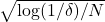
This inequality states that the true risk $R(\theta)$ is bounded by the empirical risk $\hat{R}_N(\theta)$ plus two correction terms: a geometry‑dependent term that shrinks with $\sqrt{N}$ and a confidence term that scales with $\sqrt{\log(1/\delta)/N}$ .

Here $C' = \log V_\Theta - \log V_d - \log m + d\log L_f^p$ , where $V_\Theta$ is the volume of the full parameter space, $V_d$ the volume of a $d$ ‑dimensional subspace, $m$ a lower bound on $\sqrt{\det(F(\theta))}$ , and $L_f^p$ a Lipschitz constant for the noisy model $f_{\theta,p}$ .

Limits and next steps

Our analysis relies on three assumptions that are common in learning‑theory work but may limit immediate practical use:

We assume the loss function is Lipschitz continuous and the gradients of the quantum model are uniformly bounded.
We require a positive lower bound $m$ on the determinant of the Q‑FIM; highly ill‑conditioned circuits could violate this condition.
The exponential term $\exp(C'/d)$ can become large if the parameter‑space volume or Lipschitz constant is not carefully controlled.

Future research directions include:

Designing training regularizers that directly enforce a well‑behaved Q‑FIM.
Developing quantum‑specific dimensionality‑reduction algorithms that preserve expressive power while lowering $d$ .
Empirically testing the bound on near‑term quantum hardware to validate the theoretical predictions.

FAQ

What is the quantum Fisher information matrix (Q‑FIM) and why does it matter?: The Q‑FIM measures how sensitively a quantum state (or circuit output) changes with respect to small parameter variations. Its determinant captures the curvature of the parameter landscape; a larger determinant indicates a well‑conditioned space where learning is stable, which directly reduces the complexity term in our bound.
How does reducing the effective dimension $d$ improve generalization?: All three terms in the bound become smaller when $d$ drops. In particular, the factor $\exp(C'/d)$ shrinks, and the prefactor $12\sqrt{\pi d}$ scales with $\sqrt{d}$ . Dimensionality reduction therefore tightens the guarantee and makes the model less able to fit random noise.
Is the bound applicable to noisy quantum hardware?: Yes. Our derivation explicitly includes a noise parameter $p$ through the model $f_{\theta,p}$ and shows that the bound remains valid as long as $p$ stays within a regime where the Lipschitz constant $L_f^p$ and the Q‑FIM lower bound $m$ are preserved.

Read the paper

Controlling Generalization in Quantum Machine Learning via Fisher Information Geometry and Dimensionality Reduction

References

Khanal, B., & Rivas, P. (2025). Data-dependent generalization bounds for parameterized quantum models under noise. The Journal of Supercomputing, 81(611), 1–34. https://doi.org/10.1007/s11227-025-06966-9. Download PDF

How IEEE Std 7003‑2024 Shapes Bias Management in Autonomous AI Systems

We evaluate IEEE Std 7003‑2024, showing how its bias profile, stakeholder mapping, and risk assessment improve AI transparency and fairness.

We examined the new IEEE standard for algorithmic bias in autonomous intelligent systems, highlighting its strengths, gaps, and practical implications for developers, researchers, and regulators.

TL;DR

IEEE Std 7003‑2024 provides a structured, documentation‑first framework for bias mitigation in autonomous AI.
Its bias‑profile, stakeholder‑mapping, and risk‑assessment clauses improve transparency and auditability.
Key gaps include missing quantitative metrics, limited sector‑specific guidance, and a need for conflict‑resolution mechanisms.

Why it matters

Algorithmic bias can undermine trust, exacerbate inequalities, and expose developers to legal risk. As autonomous intelligent systems (AIS) are deployed in high‑stakes domains such as healthcare, finance, and public safety, regulators and the public demand clear evidence that these systems are fair and accountable. A standardized approach gives organizations a common language for documenting bias‑related decisions, helps auditors trace how those decisions were made, and offers regulators a concrete benchmark for compliance. Without such a framework, bias mitigation efforts remain fragmented and difficult to verify.

How it works (plain words)

Our evaluation followed the standard’s five core clauses and broke them down into everyday steps:

Bias profiling (Clause 4): Developers create a living document called a “bias profile.” This record lists the data sources, known bias risks, and mitigation actions taken at each stage of the system’s life cycle.
Stakeholder identification (Clause 6): Early in the project, teams map all parties who influence or are impacted by the AIS: engineers, users, regulators, and potentially marginalized groups. The map ensures that diverse perspectives shape design choices.
Data representation assessment (Clause 7): Teams review whether the training data reflect the real‑world population the system will serve. The standard asks for a qualitative description of any gaps, though it does not prescribe numeric thresholds.
Risk‑impact assessment (Clause 8): Developers estimate the likelihood and severity of bias‑related harms, then prioritize mitigation actions accordingly. The process mirrors traditional safety‑critical risk analyses, making it familiar to engineers.
Continuous evaluation (Clause 9): After deployment, the bias profile is updated with new monitoring results, and the risk assessment is revisited whenever the system or its environment changes.

By weaving these steps into existing development workflows, the standard turns abstract ethical goals into concrete engineering artifacts.

What we found

Our systematic review of the standard, backed by case studies from content‑moderation tools and healthcare AI, highlighted three high‑impact outcomes:

Improved traceability: The bias profile forces teams to record decisions that would otherwise remain tacit. Auditors can follow a clear chain of evidence from data selection to model output.
Better stakeholder engagement: Early mapping of affected groups reduced the likelihood of overlooking vulnerable populations, which aligns with best practices in human‑centered design.
Structured risk awareness: The risk‑assessment template helped teams quantify potential harms and prioritize resources, producing more defensible safety cases for regulators.

Across the examined examples, teams reported faster compliance reviews and clearer communication with oversight bodies. However, the lack of explicit quantitative metrics for data representativeness limited the ability to benchmark progress across projects.

Limits and next steps

All inputs agree on three principal limitations:

Missing quantitative benchmarks: The standard describes what to assess but not how to measure it numerically. Without clear thresholds, organizations must invent their own metrics, leading to inconsistency.
Sector‑specific guidance is absent: Domains such that finance, criminal justice, and medical diagnostics face unique bias vectors. Tailored annexes would make the standard more actionable for specialized teams.
Limited conflict‑resolution guidance: When stakeholder priorities clash, e.g., a business’s efficiency goal versus a community’s fairness demand, the standard offers no procedural roadmap.

To address these gaps, we recommend:

Developing companion documents that define quantitative metrics (e.g., demographic parity thresholds) for common data domains.
Creating industry‑specific annexes that translate the generic clauses into concrete checklists for finance, healthcare, and public‑sector AI.
Embedding a stakeholder‑conflict resolution process, perhaps borrowing from established ethics‑review frameworks, to help teams navigate competing interests.

Future work could also explore automated tooling that integrates bias‑profile updates into continuous integration pipelines, further lowering the operational burden.

FAQ

What is a “bias profile” and why should we maintain one?: A bias profile is a living document that records data sources, identified bias risks, and mitigation actions throughout the AI life cycle. It makes bias‑related decisions transparent and auditable.
Do I need to collect new data to comply with IEEE Std 7003‑2024?: No. The standard does not force new data collection, but it does require a clear assessment of how well existing data represent the intended user population.
Can the standard be applied to small‑scale projects?: Yes. While the standard was written with large, high‑impact systems in mind, the documentation‑first approach can be scaled down; a lightweight bias profile can still provide valuable traceability.
How does the standard help with regulatory compliance?: By providing a structured set of artifacts, bias profile, stakeholder map, and risk assessment, regulators have concrete evidence of bias mitigation efforts, simplifying audits and certifications.

Read the paper

Download or view the paper

Reference

Huang, W., & Rivas, P. (2025). The new regulatory paradigm: IEEE Std 7003 and its impact on bias management in autonomous intelligent systems. In Proceedings of AIR‑RES 2025: The 2025 International Conference on the AI Revolution: Research, Ethics, and Society (pp. 1–13). Las Vegas, NV, USA. Download PDF